Shock response with SEA - What to expect?
Example of the application of SEA in shock propagation analysis.
Shock response with SEA - What to expect?
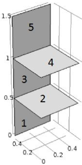
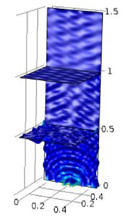
I got a chance to revisit an application of Statistical Energy Analysis (SEA) during some course work at KTH; the application of predicting high frequency shock response of plate-like structures, which I researched in my Masters Thesis one and a half decade ago. The analysed structure is shown below, comprised of five connected metal plates.
 |
 |
Shock waves in structures due to sudden release of energy are common in aerospace applications. Explosive bolts to separate rocket stages, latches and deployment of appendices are some examples. The shock load is often short in time and the frequency content of the propagating waves are high. In some cases, the analysis is performed up to 100 kHz. This requires a high element-density when using FE-methods to predict the shock wave propagation. That’s where SEA comes in to play.
Statistical Energy Analysis (SEA)
SEA was developed for analysing mid- to high-frequency acoustics and has been later on become a tool in vibro-acoustics. Instead of a calculating the deterministic responses of structures, a statistical approach is done by considering an average response of similar sub-structures. An “element” can be one of the plates in the presented structure.
A typical two-subsystem arrangement, depicted in the figure below, is commonly used to demonstrate the power flow in SEA.
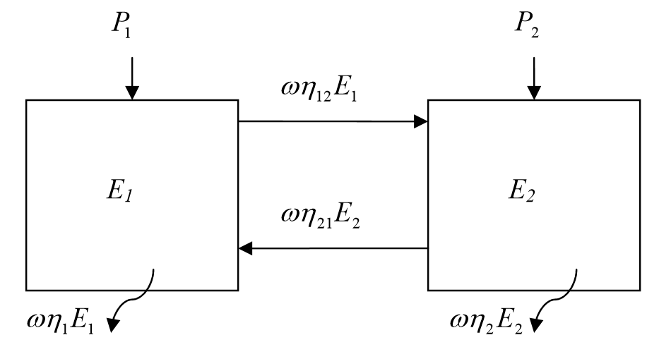
$E_i$ represents the vibro-acoustic energy of $i$:th subsystem and the power input to each system is $P_i$. Each subsystem has a power-loss, $\omega \eta_i E_i$, where $\omega$ is the analysed center-frequency and $\eta_i$ is the loss factor. The energy exchange between the two subsystems are governed by the coupling loss factor $\eta_{12}$ and the reciprocal loss factor $\eta_{21}$. The power balance for the system may be set up and written
,
,
where the modal density $n_i$ of the $i$:th subsystem has been introduced. This system of equations may be solved for the energy and the spatial averaged velocity squared may be calculated by, $v^2 = E_i / m_i $, where $m$ is the mass of the subsystem. The Shock Response Spectrum (SRS) is commonly used to evaluate the shock severity. Anyhow, let us keep it simple and stick to analysing the velocity and acceleration responses.
What to expect?
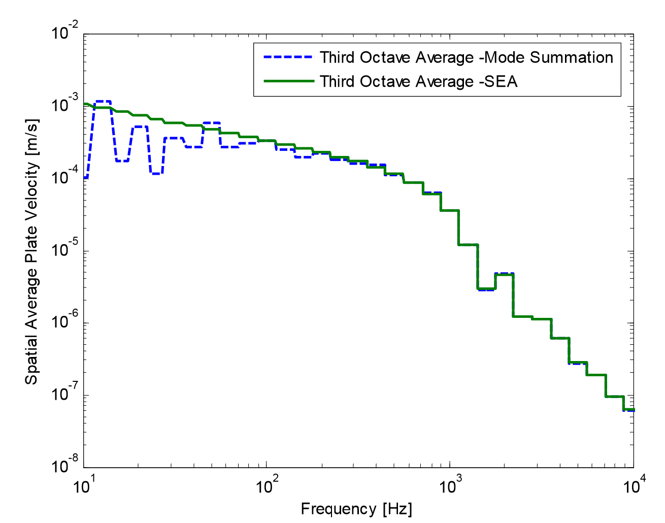
So, to the main question. What results can we expect from SEA in comparison to a deterministic approach? In SEA, there is no modal content since we only look at the spatial averaged response, based on the vibro-acoustic energy of the sub-systems. For a deterministic method, the eigen-frequencies will be visible in the low frequency range when the modes are well separated. However, as the frequency increases, the eigen-frequencies start to overlap and individual modes are hard to spot, thus, we have a higher modal density at higher frequencies. SEA is only valid at high frequencies where the modal density is sufficiently large. Let us visualize this in an example of a simply supported plate excited by a half-sine impulse of 200 $\mu s$.
The blue dotted line in the figure to the right shows the average-velocity of 30 random points on the plate in third-octave bands, calculated by the (deterministic) mode summation technique and the green line is calculated with SEA. At 3-4 kHz we see how the results converge. Thus, the modal density is sufficiently high for SEA to be valid.
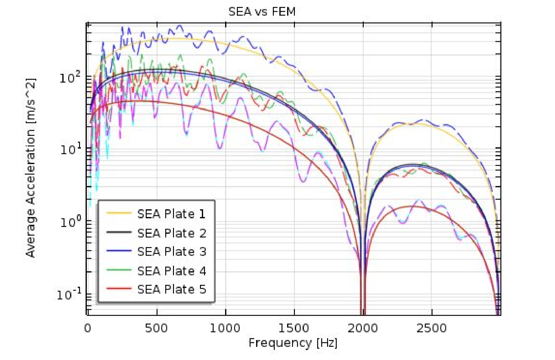
As a final example, let us excite the previously presented five-plate structure with a 1 ms Haversine impulse at the lower end of plate 1 and compare the SEA results with the results from a FE-model of the structure. In the figure below, we see the spatial average acceleration of the individual five plates, respectively. The dashed lines are from the FE-model and the solid lines are from SEA model. Here, we also see that the results converge more and more as the frequency increases and the modal density increases. We have a rather good agreement between the two methods in the high-frequency region. The high-frequency results from the FE-model is however limited by the choice of element size. The element size was chosen to give reasonable simulation time on the cost of limiting the upper frequency range. Nevertheless, this is where SEA can take over, showing how the two methods can be used in conjunction.
Conclusion
SEA is a statistical approach by considering an average response of similar sub-structures and is only valid at high frequencies where the modal density is sufficiently large. Individual modes are not considered in the low-frequency region as compared to deterministic approaches. SEA is a suitable method for high-frequency shock analysis and a good complementary tool to FE-methods.